Curves and Ruled Surfaces over Curves
Curves in Pycao are always parametrized curves. They are used:
for a film or an animation : the camera and the point you look at move on curves
in the construction of objects : Lathe objects, and ruled surfaces
There are three types of Curves :
polylines
bezier Curves
piecewise curves which are obtained by gluing pieces of curves
Notations for the control points
Polylines and Bezier Curves are defined by control points. The list used to define the control points may be simply the list of points you use. We call it the list of absolute positions. But you can also include vectors in the list, to indicate that your input is the difference of coordinate with the previous point. For instance, suppose you have your list of control points
l=[p0,p1,p2,p3,p4,p5]
with
p4=origin
p5=origin+X+2*Z
then, you could alternativly use for the list of control points
l=[p0,p1,p2,p3,p4,v5]
with
p4=origin
v5=X+2*Z
You don’t need any special declaration. When pycao encounters a vector rather than a point, it knows that you are talking about the relative position from the previous point. For instance, the following three lists correspond to the points on a plane square. The first list indicates absolute positions, the second list relative positions, the third one is a mix.
l1=[origin, point(1,0,0),point(1,1,0),point(0,1,0)]
l2=[origin, X,Y,-X]
l3=[origin,X,point(1,1,0),-X]
Polyline and Bezier Curves
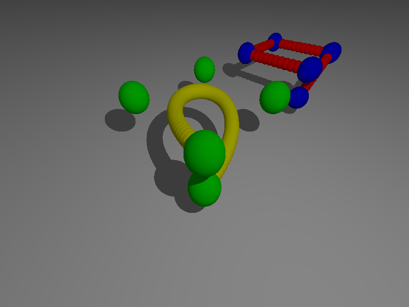
The following sequence builds the basic usable curves, namely a Bezier curve and a Polyline. Since a curve is infinitly thin, it is not possible to see it even if camera.filmActors=True. We use the method show() to add spheres along the curve to visualize it. The options of show() allow to choose a different color for the control points and for the sphere along the curve.
ground=plane(Z,origin-Z)
ground.colored("Gray")
curve1=BezierCurve([origin,-X+Y,X+Y,X-Y,-X-Y-.5*Z])
curve1.show() # use default arguments
curve2=Polyline([origin,-X+Y,X+Y,X-Y,-X-Y-.5*Z])
# For the polyline, we don't use the default options
curve2.show(radius=0.1,steps=50,color="Red",color2="Blue")
curve2.translate(2*X+2*Y+0*Z)
Interpolation and Piecewise curves
Usually we want a smooth interpolation curve. Thus neither the Bezier curve ( it passes close to the control points, but not exactly through the control points) neither the polyline (not smooth ) are suitable.
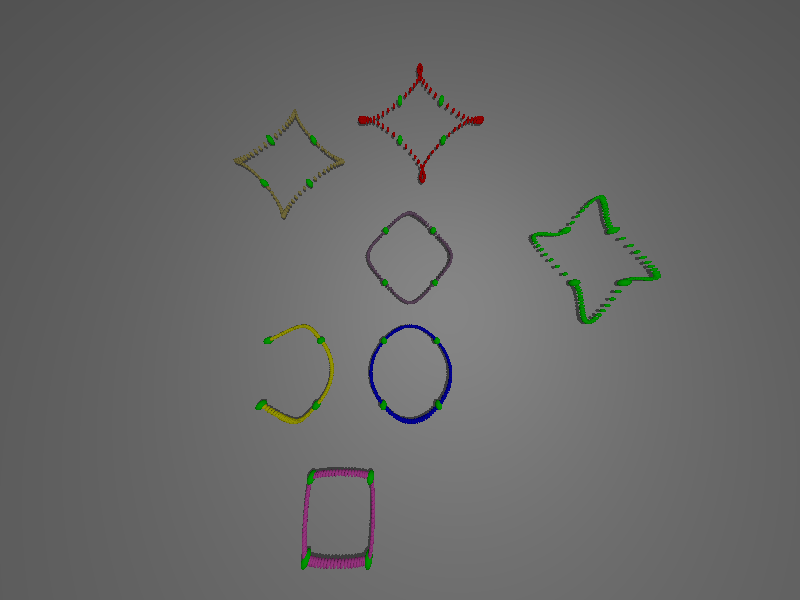
To solve this problem, pycao offers an interpolation curve which does the job. It is built from several Bezier Curves joined together. If the option closeCurve=True, Pycao will add a last point in your list coinciding with the initial point and will make a smooth junction. As a result, the curve is closed and appears smooth at the junction point between the start and the end of the curve.
controlPoints=([origin+.1*Z,X,Y,-X])
curve1=PiecewiseCurve.from_interpolation(controlPoints).show(radius=0.03)# color Yellow
curve2=PiecewiseCurve.from_interpolation(controlPoints,speedConstants=[.24,.24],closeCurve=True).show(radius=0.03,color='SpicyPink').translate(-2*Y+X)
curve3=PiecewiseCurve.from_interpolation(controlPoints,closeCurve=True).show(radius=0.03,color='Blue').translate(2.2*X) # speedConstants=[.45,.45]  by default
curve4=PiecewiseCurve.from_interpolation(controlPoints,speedConstants=[1.5,1.5],closeCurve=True).show(radius=0.03,color='Violet').translate(2*Y+2.2*X)
curve5=PiecewiseCurve.from_interpolation(controlPoints,speedConstants=[3,3],closeCurve=True).show(radius=0.03,color='Bronze').translate(4*Y-.5*X)
curve6=PiecewiseCurve.from_interpolation(controlPoints,speedConstants=[4,4],closeCurve=True).show(radius=0.03,color='Red').translate(5*Y+2.5*X)
# In the following line, the curve has 4 points + one point added by Pycao to close the curve, so the speed vectors have 5 entries
curve7=PiecewiseCurve.from_interpolation(controlPoints,approachSpeeds=[2,2,2,2,2],leavingSpeeds=[0.4]*5,closeCurve=True).show(radius=0.03,color='Green').translate(2*Y+6*X)
All the curves above have been made with the same list of control points, shown in green. What makes the difference is the speed of the curve at the control points. When the curves goes slowly through the control point, the change of direction is fast. On the other hand, if the speed is hign, the curve keeps its direction a bit longer. On the picture, the small speed is for the pink curve. The speed is so small that the curve looks like a polyline. The default speed is for the blue curve. The highest speed is on the top, for the red curve, where the speed is so high that the curve goes too far and needs to come back to go to the next point.
The direction of the vector speed at the point p_i is parallel to the vector p_{i+1}-p_{i-1}. It is only the norm of the speed vector that you control with the speed parameters. For each control point, you can choose two constants, a constant to control the speed used when the curve approaches the control point, and another constant for the speed used when the curve leaves the control point.
On the right part of the picture, the green curve is a curve where the approching speed is different from the leaving speed. For the other curves, the approach speed is equal to the leaving speed.
Choosing the speed for each control point may be tedious, thus you can control all the points simultaneously using the parameter
speedConstants=[approachingSpeed,leavingSpeed]
If you prefer, you can control the points individually using the parameters
approachSpeed=[speedAtPoint0,speedAtPoint1,...]
leavingSpeed=[speedAtPoint0,speedAtPoint1,...]
Ruled Surfaces built on curves
Ruled surfaces are a generalization of Prisms and extruded surfaces.
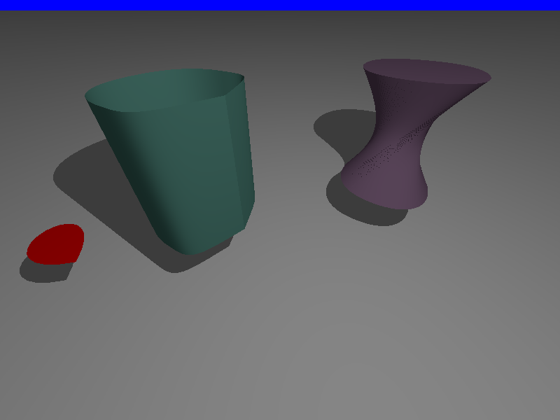
It is possible to fill a closed curve to get a surface. For instance, if we fill a circle, we get a disk. The calling sequence is RuledSurface.fromCurveFilling(curve), as illustrated in the red example below.
It is possible to construct a ruled surface by joining the points C(t) and D(t) of two curves C and D. The following example illustrates that the result depends on the parametrization of C and D . The violet join uses curves similar to the green join, but with a different parametrization equivalent to a rotation of the bottom curve. It looks like we have applied a torsion to an aluminium can. The violet join also illustrates that we can optionally add caps at the extremities of the join.
ground=plane(Z,origin-Z)
ground.colored("Gray")

#Filling a Bezier curve in Red
curve0=BezierCurve([origin,-X,+Y,+X,origin])
curveFilling=RuledSurface.fromCurveFilling(curve0,quality=2)
curveFilling.colored("Red")
curveFilling.translate(-2*X)

# The green join
curve1=PiecewiseCurve.from_interpolation([origin,-X,+Y,+X,origin])
# Remark the non smooth join.
curve2=curve1.clone().translate(1.5*Z).named("Courbe2")
tube=RuledSurface(curve1,curve2,quality=8)
tube.colored("HuntersGreen")

#The violet join
# Now, for curve3, to get a smmooth join, we suppress one point in comparison to curve 1,
# and we add the option closeCurve=True.
curve3=PiecewiseCurve.from_interpolation([origin+3*X,-X,+Y,+X],closeCurve=True)
curve4=curve3.clone().translate(1.5*Z)
def g(t):
   return (t+0.35) %1
curve3.reparametrize(g)
tubeWithRotatedBottom=RuledSurface.fromJoinAndCaps(curve3,curve4,quality=5)
tubeWithRotatedBottom.colored("Violet")
Lathe
The lathe object is defined by rotating a curve located in the half plane z=0, x>0 around the Y-axis.
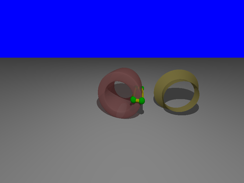
curve=PiecewiseCurve.from_interpolation([origin+X-Y,.5*X,+2*Y,-.5*X],speedConstants=[.24,.24],closeCurve=True).show()
Lathe.fromPiecewiseCurve(curve).rgbed(.8,.4,.4,.5)

curve2=Polyline([origin+X+2*Y,.5*Y,.5*Y+.5*X])
Lathe(curve2).colored("Bronze").translate(4*X-2*Y)
Plane(Z,origin-1.5*Z).colored("Gray")
# The curve is assumed to have points of the form [0,y,z]